Five Flute - Engineering design review platform for modern hardware teams

Before we get started

This article will help you diagnose and resolve issues in your finite element models, but that's not the only kind of issue you will find in product development! So we've built Five Flute to help you with all the other issues you will encounter as you design, build, test and deliver great hardware products. Check it out!

Motivation

I’ll start this post with a troubling observation from my career as a practicing mechanical engineer and product designer.

The vast majority of engineers I have worked with have not been properly prepared to evaluate the quality of FEA data. And yet the companies they work for and the colleagues they work with continually rely on that data to make critical decisions about the products and services they develop.

And it’s no wonder when you consider the widespread usage of computer aided engineering (CAE) tools and the complete lack of formal FEA training in undergraduate engineering programs.

Finite element modeling is an extremely powerful method in the mechanical engineer’s tool kit. With the advancement of meshing tools, and the inclusion of FE packages in modern CAD tools like Solidworks, FE modeling has become ubiquitous. Gone are the days when stress analysts and engineering specialists were solely responsible for building finite element models. Increasingly FEA has become a generalist tool for engineers and product designers and it is expected that design engineers should be capable of running their own stress analysis and building their own FE models. The downside of this is that many engineers are learning FEA on the fly without a foundational understanding of the method, risking expensive or dangerous mistakes in the products and machines they design.

The goal of this guide is to provide generalist engineers with enough foundational knowledge of FE modeling to feel comfortable leaning on the method for most common engineering problems they will encounter as designers. As we often do in the Five Flute Engineering Guide we will take a first principles approach, first reviewing the mathematics behind FEA, connecting the mathematics with model setup, establishing practical guidelines for model setup and finally discussing the interpretation of results. We will not be focusing on specific codes, solvers or software packages, but rather on foundational principles that extrapolate to any CAE package you might use.

Note: Much of this post will focus on structural analysis problems, but the general guidance extends to other domains where FEA is used.

Fundamentals

What is FEA?

Finite Element Analysis (FEA) is a numerical method used to solve boundary value problems. A boundary value problem is mathematically represented as a system of differential equations where the solutions and derivatives are known at certain points (or boundaries). These solutions are described by boundary conditions. To put this in terms of a mechanical engineering problem we can use the example of a simple beam with clamped ends.

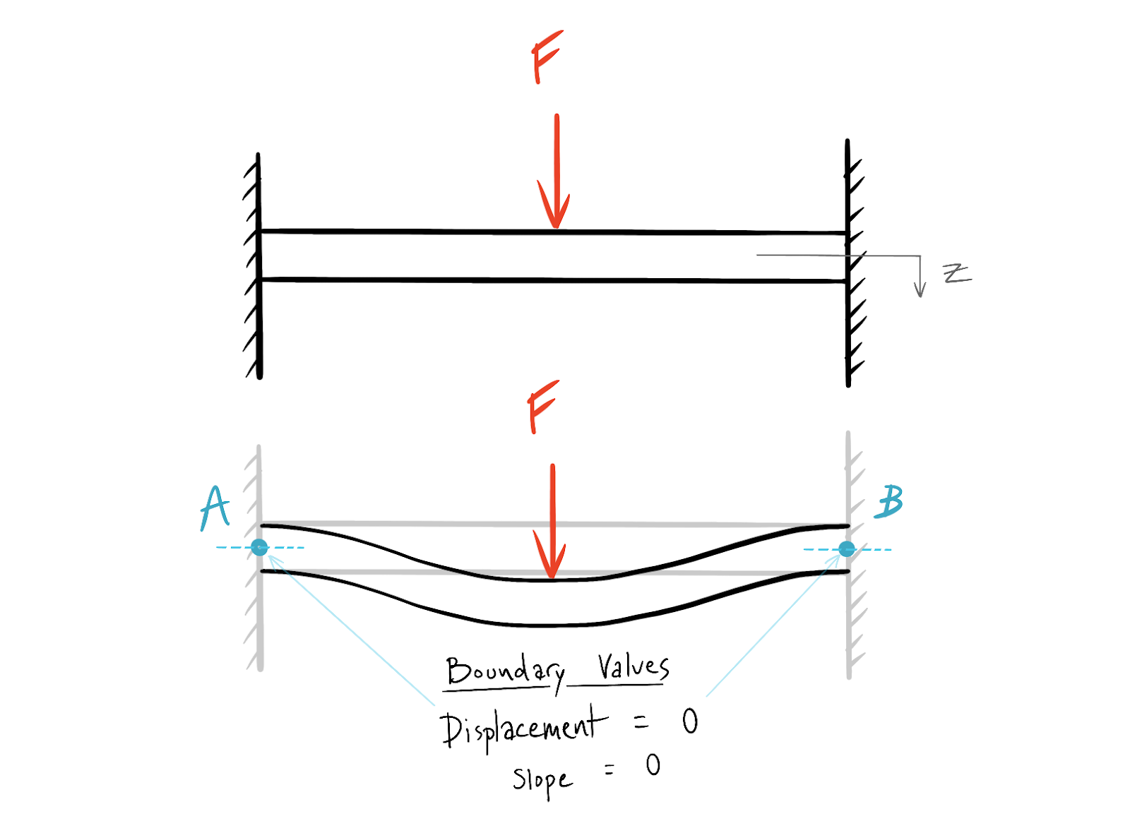
The boundary conditions of the beam are described by the “clamped” condition of each end, meaning there can be no displacement or curvature (derivative of displacement) at either end of the beam.

FEA is a method of solving these boundary value problems over continuous domains (like solid bodies) through the assembly of continuum elements. The solution is obtained by representing the structure using subdomains or “finite elements.” In the case of structural analysis, the field variable we care about is generally displacement. This field variable is represented by a set of assumed functions and nodal values over each element. The individual elements are then assembled into a system of algebraic equations that can be solved for the nodal values. In general, loading and boundary conditions are represented by prescribing nodal forces and displacements respectively.

If the above explanation made you even more intimidated and confused about how FEA works don’t worry! It is not absolutely necessary to understand all of the math going on under the hood in order to build good FE models using modern CAE tools. We asked “What is FEA?” in order to highlight how our choices as engineers impact the problem setup and solutions we get from our models. There are three key things to take out of our brief explanation of FEA above:

We are discretizing the domain into chunks, called “finite elements.”
Loads and constraints (conditions) are represented at nodes.
We are assuming functions to represent displacement (and stress, strain, etc..) over the domain.

Discretization and Nodes

Discretization means we are dividing up a continuous domain (ex: the 3D geometry of a machine part) into discrete chunks. Each chunk is represented by an element. The distribution of elements is defined by the mesh. There are many different types of elements, and their usage depends both on the type of problem we are representing and the type of solution we expect. The simplest element is just a 1D 2-node bar element.

The nodes are defined by their location in space, representing degrees of freedom of a field variable. For structural analysis problems these degrees of freedom are spatial displacements in x, y and z. For thermal problems the degree of freedom we care about is temperature.

The important thing to remember is that the system of equations running in the background of your FEA tool is solving for the field variables at the nodes only. In between the nodes the field variables are interpolated. In other words, the solver uses a function that you specify to guess at the values of the field variable in between the nodes. That's where our choice of element really comes into play.

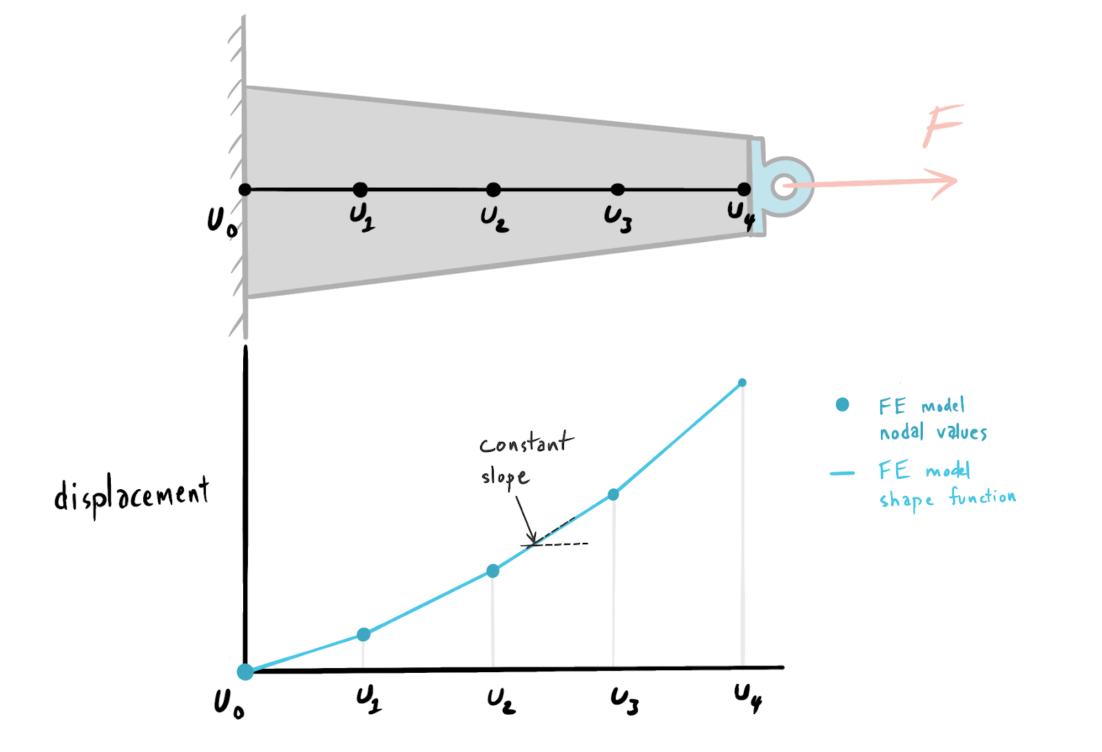
Returning to our 1-D bar element, we can use this element in an example structural analysis problem. Let’s consider a tapered bar under tension.

We can use the 2-node bar element to represent this tapered bar as a series of four finite elements where each element has a single degree of freedom in the x direction. We will use the field variable u to represent this displacement. In order for this model to work it must satisfy three conditions.

Compatibility. Connected ends of adjacent springs must have the same displacements. This means that nodes shared by connected elements must have the same field variable values.
Static Equilibrium. The resultant force at each node is zero. We are saying that forces between nodes must balance out, basically Newton’s third law.
Constitutive Relation. We need some way to describe how the element will behave under load. For the 1-D bar example using a 2-node element the constitutive structural relationship is a Hooke’s law. Each element behaves like a spring.

Putting all of this together we end up with a representation of the tapered bar as four series connected springs with an average element stiffness derived from the area of the tapered beam at the midpoint of each element and the length of the element.

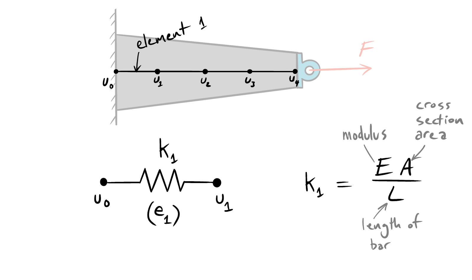
Tapered beam representation with first element constitutive relationship and stiffness.

Direct Stiffness - Element Behavior

For the sake of demonstrating what is happening behind the GUI of your FEA program (Solidworks, Ansys, Abaqus etc...), we will review the Direct Stiffness Method for FE modeling. Note: there are other methods, but direct stiffness provides a nice introduction that we can explain using our tapered beam example.

The basic idea is to build up the behavior of the whole system from the individual elements. Direct stiffness accomplishes this by relating nodal forces to nodal displacements by way of element stiffness for all elements. We know that there must be equilibrium across our 1-D bar element (condition 2, static equilibrium), and we know the stiffness of this element (condition 3 - constitutive equation is Hooke’s law with axial stiffness of a bar). Putting together the equilibrium condition and the constitutive equation yields the following formulas that describe the element behavior.

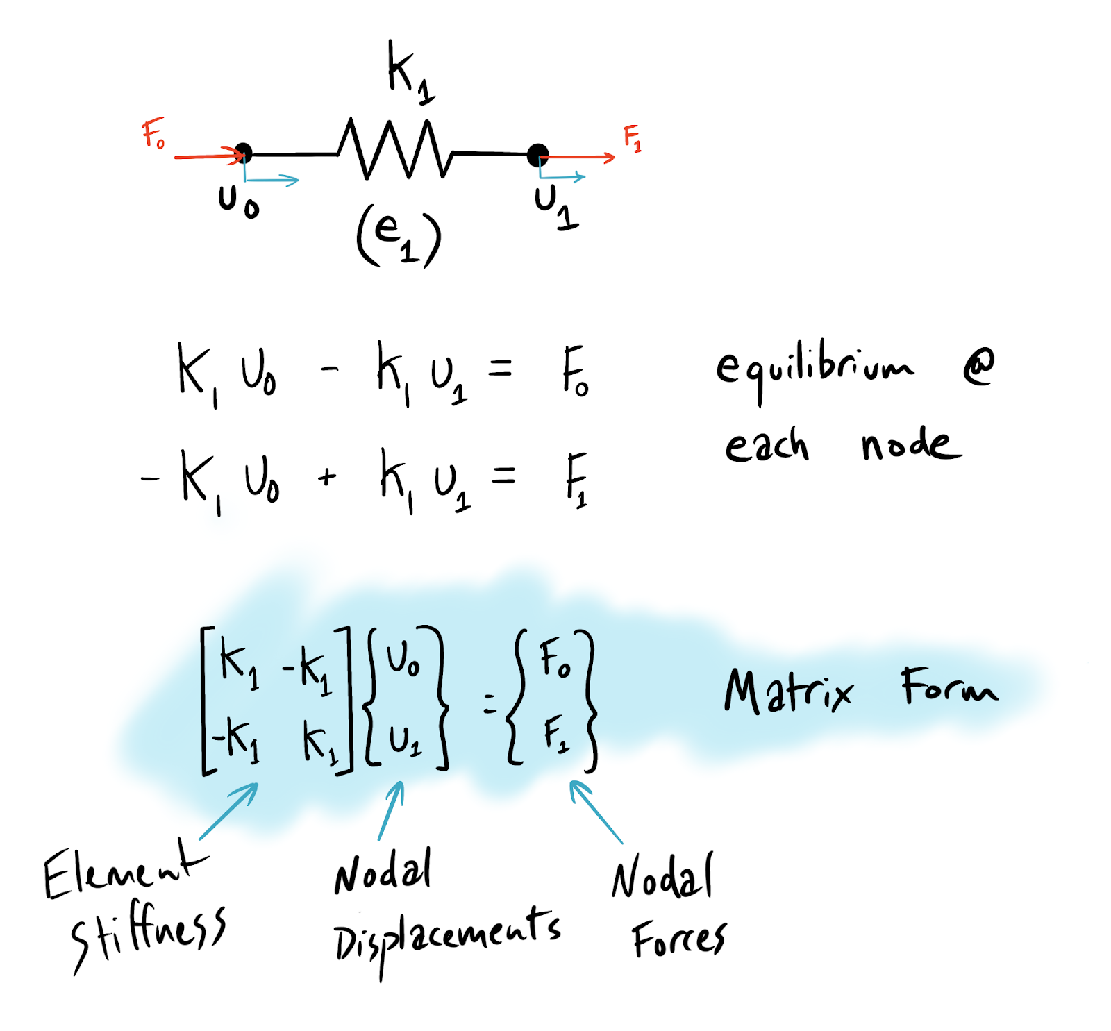
Direct Stiffness - Global Behavior

The beauty of the method is that you can perform simple repetitive calculations for each element, then sum up all of the elements into a complete picture of the system using superposition. For our tapered bar example, we would end up with a system of equations that looks similar to the form used for each individual element. Superposition allows the global stiffness matrix to be constructed from the individual element stiffness matrices.

Applying Loads and Constraints

Now that we have a representation of the continuous bar as finite elements, we need to apply the boundary conditions. These boundary conditions are representative of the loads and constraints on the system. The constraints are fairly simple in this case since the left side of the bar is fixed, so the left side of element number one is fixed, meaning the field variable for displacement (u_0) must equal zero. Loading can be represented as a point load (f_4) on the right node of the fourth element.

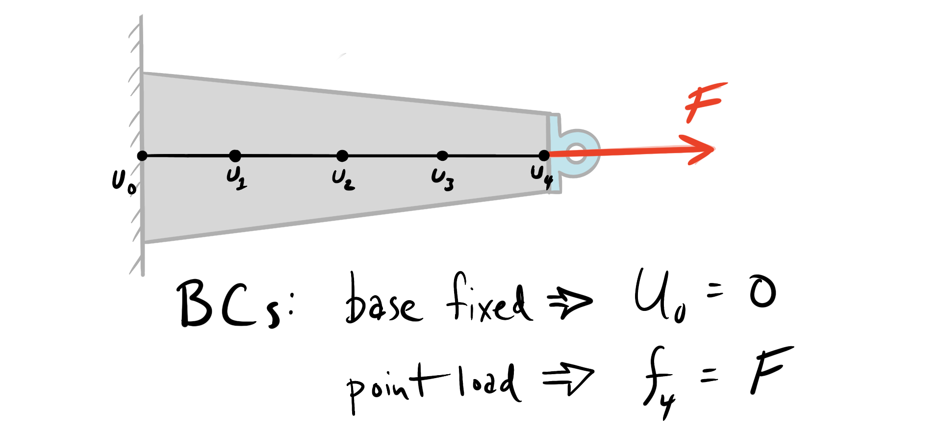
Adding loads and constraints gives the FE code enough information to solve a large system of equations.

Note: For the direct stiffness example, adding loads and constraints keeps the stiffness matrix from being singular (determinate of K must not equal zero), allowing nodal displacements to be solved by inverting the stiffness matrix. Cambridge University has a wonderful walk through of the direct stiffness method that steps through the math with clear examples: https://www.doitpoms.ac.uk/tlplib/fem/intro.php

Shape Functions

Once nodal displacements are known, there is still the challenge of representing the stress in all other locations that are not nodes. This is where shape functions (sometimes called basis functions or interpolation functions) become essential. Shape functions effectively fit the field variables between the nodes. They are a property of the elements we choose, and have big implications on the type of response we can expect. Returning to our 1-D bar example, we can think of shape functions as a simple curve fit on the nodal data. With only 2 nodes in a linear element, we can only represent linear changes in stress. The linear element solution will show a constant rate of change of displacement between nodes as follows.

Discretization Error

Discretization error is inherent to the majority of numerical methods, FEA included. A simple way to understand discretization error is through Reimann Sums. A Reimann sum is an approximation of a definite integral using rectangles. Each rectangle is a discretization of a continuous curve and has an associated error. As the rectangle width decreases, the error converges, but never disappears entirely.

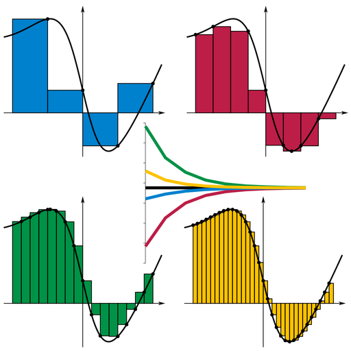
Reiman sum for definite integral calculation. Convergence shown as rectangle width decreases. https://en.wikipedia.org/wiki/Riemann_sum#/media/File:Riemann_sum_convergence.png

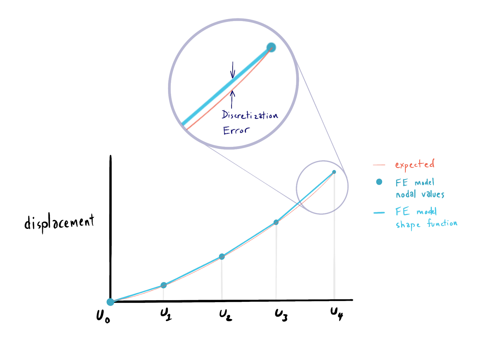
The same behavior happens with FEA. As element and/or node count is increased, the error of models decreases, but at the cost of more complicated calculations. This is the fundamental reason that mesh sizing relative to feature sizing matters. We will discuss this in greater depth in the model setup portion of this guide.

To put discretization error in a finite element context we can return to our tapered bar example. By observation we know that with a continuous tapered bar, we should expect that there will be a smooth change in the displacement and stress in the bar under tension. Plotting the FE solution to our tapered bar example alongside what we would intuitively expect as an answer reveals the discretization error inherent in our 1-D element choice.

Models are representations only

We went through the math of FEA and what is happening “under the hood” so to speak, but we still haven’t touched on the modeling aspects of FEA directly. Like other models we use as engineers, FEA is a representation of some real world phenomena. It is not telling us “the truth” and should not be interpreted as such. With the right assumptions, careful setup and diligent interpretation our finite element models can tell us a useful story.

What is a Finite Element Model?

It can be helpful to think of FEA as a multi stage process of filtering through which a real world engineering problem is converted into useful results. The goal of each filtering step is to remove superfluous or unnecessary information while preserving an accurate and useful representation of some physical phenomenon. This filtering process is represented in the figure below.

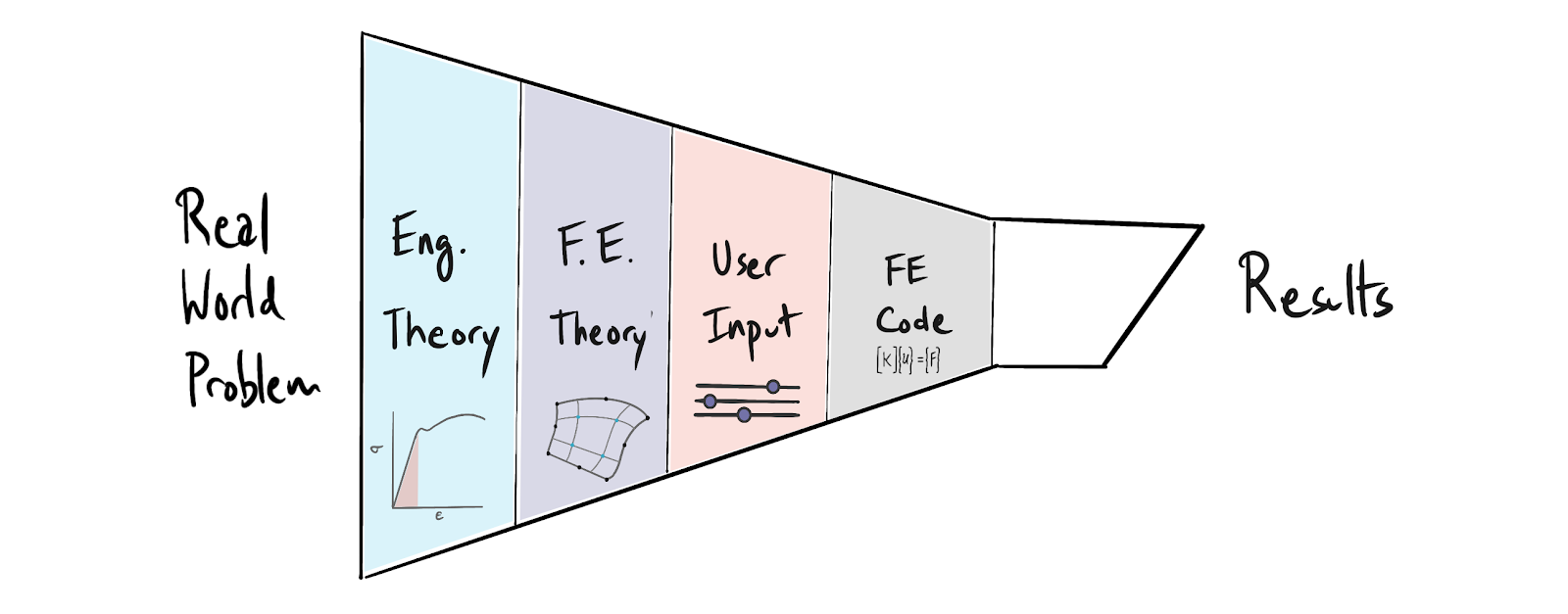
The first filter in this multi stage process is engineering theory. Engineering theory allows us to create a valid mathematical representation of a real world problem with an incomplete subset of information. The second stage is finite element theory. This is what we reviewed earlier in this post. Finite element theory introduces its own set of approximations and compromises on top of engineering theory. The third stage is user input. This is likely the most important and constraining filter in the modeling process. If we as engineers do not translate our understanding of the real world problem into valid and appropriately representative inputs (through element choice, meshing and boundary conditions) then our models will return an approximately correct solution to the wrong problem. The next stage is the finite element code itself. This is the actual implementation of the finite element theory. The code returns results, which must be interpreted in order to be useful.

Model Setup

Now that we have a basic understanding of the math behind FEA as well as a framework for thinking about FE models generally, we can dive into practical guidance for building useful models. We will not be focusing on specific finite element programs or interfaces, so this guidance should be broadly applicable. There are a few key questions that it helps to think through with every finite element model you create, regardless of the real world problem you are trying to solve.

Complexity Reduction

We can expect that sources of error will increase exponentially with the complexity of our models. Also, our ability to reason about these models and to extract useful interpretations out of the resulting data is inhibited severely by model complexity. You should strive to build models with only as much complexity as you are able to understand and qualify. This principle applies broadly to analysis outside of finite elements. A low resolution correct answer is more useful than a high resolution incorrect answer. Accordingly, the first question to ask yourself is, how can I reduce the complexity of my model to a level where I can have high confidence in the results? We will step through a few techniques for complexity reduction.

Defeature

CAD models and input geometry should be defeatured to reduce the size and complexity of the mesh. As you begin to build your intuition about load paths (or temperature gradients etc...) you will be able to see what features can be removed or simplified. If a feature is unlikely to contribute to the output or is sufficiently far away from areas of interest you should consider defeaturing. In some cases defeaturing can mean eliminating this geometry altogether (see bending shaft example below).

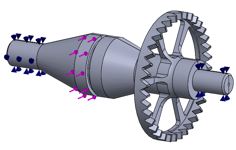
Full Featured CAD geometry of part

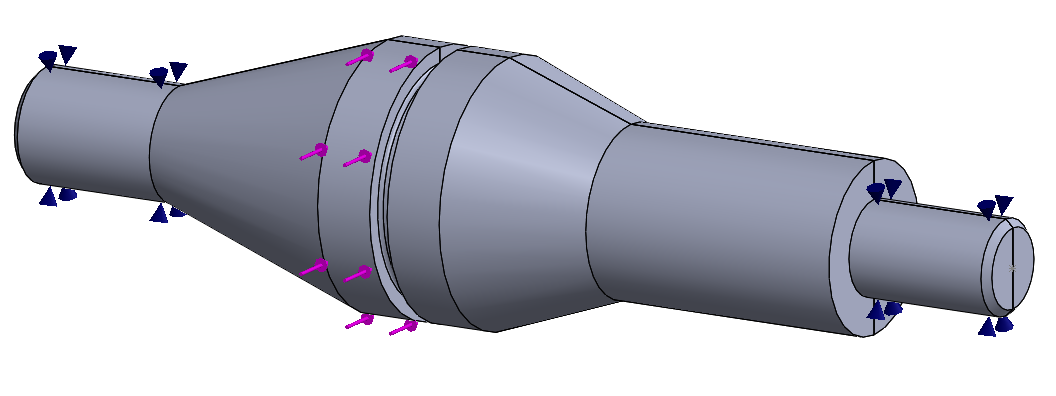
Defeatured for analysis. Note the gear feature is removed entirely due to the lack of contribution to bending induced stress in the main shaft body.

In other cases the complicated geometry can be represented by equivalent but simpler geometry. This is largely experiential, but you can approach building your intuition by testing simple models with and without certain features.

Look for Symmetry

In many cases the parts we design already have some form of symmetry by virtue of part function or manufacturing process. The symmetries we care about from an analysis perspective are typically rotational, translational or mirror symmetry. Rotational and translational symmetry can sometimes be used to reduce 3-D problems to 2-D solutions.

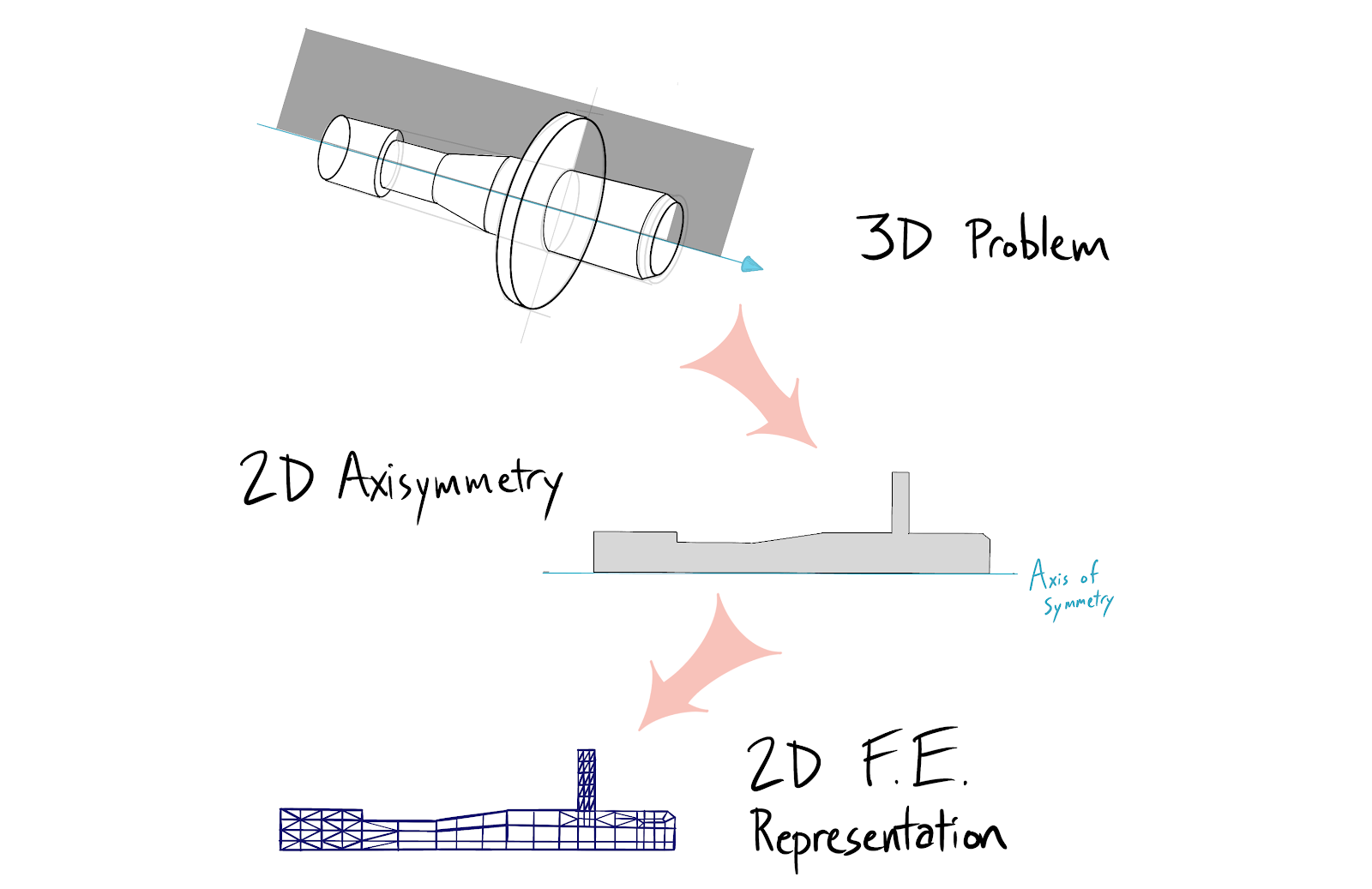
Mirror symmetry can often be used to cut a 3-D model in half or a quarter of its original size. This allows us to win back computation time and trade this time for either greater element density or the usage of higher order elements (more nodes per element with higher order polynomial shape functions). Remember that the accuracy of your choice to exploit symmetry depends on boundary conditions as well. If the loading and constraints also share the geometric symmetry it is less likely (but not guaranteed) they will be misrepresented by symmetric reduction. If the material or process introduces some orthotropic or anisotropic behavior your symmetry assumption may be invalidated in ways that are challenging to predict or interpret.

Component Contribution Analysis

For assembly studies a system should be broken into sub components with boundary conditions developed for each individual analysis. These boundary conditions should represent the component’s interaction with the rest of the system. Forcing you to consider the contribution that each part makes to the overall system will provide a baseline for evaluating the quality of the final system model should you decide to construct a multi part contact model. This will take longer, but will give you a way to calibrate your expectations and bound your interpretations of more complex models.

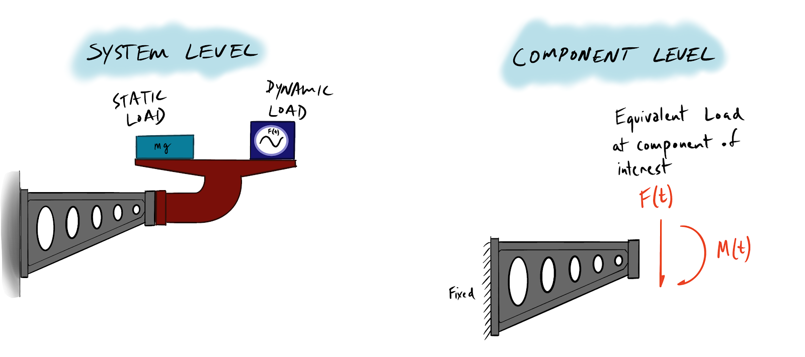
Assumptions

The second key question is, what assumptions am I making in this model? It is a best practice to articulate and document your assumptions along with their expected effect. Some of the assumptions inherent to FE models are material properties, geometry, element selection and density, boundary conditions and FE code accuracy. Until you have solid experience you should not skip this step even for the simplest of models.

Boundary Condition Development

The third key question is how can I translate the real world forces on the system being modeled into representative boundary conditions? This is a non-trivial task which can be divided into applying loads and representing constraints. It is useful to think about the proximity of both loads and constraints to the areas of the model where we are most concerned with field variable results. You should have an expectation of where displacement, strain and stress are most critical and identify where these regions are with respect to your loads and constraints. Saint Venant’s principle applies here and can be used to reduce the complexity of loads (ex: from pressure distribution to point load, or from non-linear distribution to uniform distribution) and constraints alike.

The illustration below shows a cantilever beam with a hole through the beam flange, near the fixed end of the beam. This example shows how a non-linear pressure distribution at the beam end can be translated into an equivalent point load acting at the centroid of the pressure distribution.

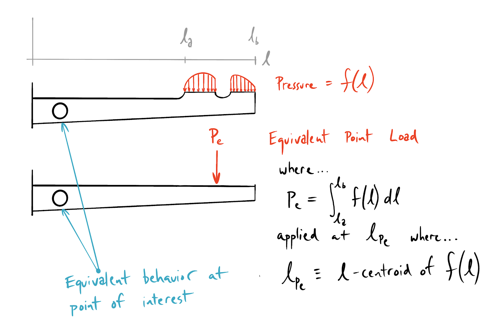
A point load is significantly easier to input into a finite element program. Because of the large distance between the load and the potential failure point of the beam, any higher order behavior at the point of loading will be resolved by the time it is reacted at the base. Saint-Venant’s principle dictates that the two systems will have equivalent states of stress near the hole.

Meshing

The fourth key question is, how will my element and meshing choices impact the model results? To answer this question you need to have a basic expectation of model results before you begin meshing. Different element types carry different tradeoffs between computational cost and their ability to represent field variable distributions. With the rise of auto-meshing tools that use the tetrahedral element you should be wary of mindless meshing. It is very easy to rely on stock meshing tools without making adjustments. While it is not impossible to develop accurate models using tet elements, their inclusion as the default choice in many FE programs can prevent users from ever considering element choice in the models. A detailed treatment of element choice is well beyond the scope of this post. We recommend that engineers familiarize themselves with first and second order tetrahedral, hexahedral and shell elements. A good overview of element architecture can be found in the documentation for the open source FE program Calculix.

Results Interpretation and Model Validation

The final stage of any analysis is to interpret the results. With FEA this is not always a simple task, precisely because the method allows us to investigate increasingly complex problems where our intuition may break down. We can achieve good results by being consistent in the ways we check and interpret our models.

'Sniff Test'

Despite model complexity, intuition and engineering judgment still play a large role in interpreting results for FEA. The first thing to ask yourself when interpreting results is “does this feel right?” Does it look like you expect it to look? Where are the peak stresses and strains? Will it fail? How much displacement were you expecting?

Analytical Validation

Once you have passed the sniff test, it is important to find some other means of model validation. Analytical validation involves finding hand calculations that approximate your FE modeling problem. If possible, finding both a conservative underestimate and a conservative overestimate to bound your problem space can provide a framework for results interpretation that can further guide our intuition.

Bounding solutions can be accomplished through grossly simplified geometry and/or loading conditions that can be worked through with a closed form solution. Shigley’s and Roark’s Formulas for Stress and Strain are great resources for finding closed form bounding solutions.

Empirical Validation

With complex problems requiring very accurate finite element representations, a physical test may be necessary. Empirical validation can involve everything from full scale tests of the product or part in question all the way down to scale models, reduced complexity tests of sub components, or even test specimens/coupons for material properties only. As with all physical testing it is essential to be explicit about what is being tested. Construct a test plan and design a test that answers your questions with the simplest possible setup.

In this case, the requirements for your test are driven at least partly by where you expect error in your finite element model. Are you unsure of the accuracy of your material representation? Maybe an Instron test of tensile specimens from the manufacturer will yield better stress strain data for your FEA. If stiffness or vibration is a concern, perhaps a scale model can validate your approach while keeping costs down. If you are developing a multi-part contact model with very elastic components (ex: rubber bumpers) it might make sense to develop a separate FE model and physical test just to validate your ability to predict rubber behavior under comparable loads before proceeding with the full assembly analysis.

The most cost effective approach may be a blend of empirical testing and analytical validation combined with problem space bounding. Creativity in test design can pay dividends here. In general this is too subtle and complex a space to provide easy rules of thumb other than to be creative, aim for simplicity and be conservative.

Model Error and Correction

If your models are not agreeing with your intuition or your empirical validation efforts, you will need to discover and characterize the error sources. Again, reducing your model’s complexity limits the number error sources to investigate. We can get a head start on error checking by identifying common errors and associated mitigation strategies.

Errors of Assumption

Earlier we mentioned some of the common assumptions inherent to FE modeling. When your results look strange interrogating your assumptions is a great starting place or error discovery and correction. A few example assumptions and associated errors are discussed below.

Symmetry not Representative

Assumptions of symmetry can be invalid even when loads and boundary conditions are symmetric. This is most likely to occur in shock and vibration analysis as well as buckling. Using modal analysis as an example, the root cause is that constraints imposed to enforce symmetry conditions can sometimes prohibit certain anti-symmetric mode shapes. It is also possible that even though input loads and constraints are symmetric, the system might exhibit a symmetric response about a different axis of symmetry than the one chosen to reduce the domain.

Material not representative - process variability

Like all manufacturing processes, material production has variability. The degree to which this invalidates your material representations in simulation is a function of the process variance. You may need to make additional assumptions or use physical testing to account for the effects of stochastic behavior of real world problems. Another method for dealing with this variance is to establish conservative inputs based on statistical inference. Monte Carlo simulation is a great way to deal with stochastic processes or other random variables in your models. For a primer on Monte Carlo simulation check out the Five Flute Engineering guide Introduction to Monte Carlo Methods for Mechanical Engineers.

Material not representative - near yield behavior

If you are running a large deformation simulation with plastic deformation, you may have to represent your material strength differently. Different FE codes may handle this differently, but you should understand if you need to input true stress/strain data or engineering stress/strain data. Developing models for arbitrary large displacements requires careful consideration of material properties in both elastic and plastic regions.

Material not representative - isotropic vs anisotropic

Material homogeneity is a very convenient assumption. Earlier we spoke of process variability, or the homogeneity of material properties across a population of equivalent material specimens. In addition to population level variance you may need to consider specimen level heterogeneity of material properties. Imagine that you have designed some parts to be machined from precipitation hardened extruded aluminum. It is possible that the extrusion process has introduced some anisotropic material properties (ex: grain direction at the material surface is influenced by friction with the extrusion die). This may introduce another random variable of local material strength into your real world problem. If you design forged parts, isotropic material models will not take into account grain direction and material hardening induced by the forging process. In some cases these additional material properties can mean the difference between reliable usage and failure.

Material not representative - internal stress states

Similarly to our anisotropic vs isotropic assumption, it is common to ignore internal stress in parts we design. In reality there are many different sources of internal stress variance related to manufacturing processes. This is particularly important for fatigue analysis because residual compressive stress can impact fatigue life significantly. Processes like shot peening induce compressive stresses in a component’s surface thereby increasing fatigue life. If you have secondary processes that impact stress states they may need to be considered.

Material not representative - coatings and platings

Coatings and platings may change you material behavior under certain loading conditions. Your material representation is impacted by the type of problem and analysis you are conducting. For example, anodizing aluminum is likely to have a negligible effect on yield strength, but a dominant effect (12 - 30%) on fatigue life. Understanding how your coatings and platings impact your material properties is a prerequisite to developing trustworthy FE models of these components.

Geometry not representative

What you design in CAD and what you end up with in real life are not the same. Never forget that your CAD geometry is itself an assumption that may need to be challenged. This is particularly true for the development of representative boundary conditions in contact stress models where small changes in geometry can result in large differences in Hertzian stress.

Model Setup Errors

Our errors of assumption were primarily related to engineering theory. The next filter is finite element theory, and the manner in which we set up our models impacts the types of results that are possible. You can think of model setup error as mistakes associated with the translation of real world forces and constraints into appropriate boundary conditions that we can feed into our FE code. This process is always reductive and it is quite easy to throw out the right information and keep the wrong information. When the solver runs and a pretty picture pops up on your screen, don’t trust it until you’ve interrogated your model setup.

Incorrect Element Selection

The key to element selection is understanding that different element types are better suited to representing different states of stress. Look at the critical regions in your model and understand how the field variable values you are observing relate to the types of field variable distributions that you element is capable of representing. If you are using first order elements you may be over representing stiffness due to shear locking. If you are modeling materials with poisson’s ratio near 0.5 such as rubbers, you may be over representing stiffness due to volumetric locking.

The Tips and Tricks section of this guide will cover how to prevent these errors in practice, but for now it is essential to be familiar with how element choice relates to real world phenomena.

Incorrect Element Density

The fundamental tradeoff of discretization is one of accuracy vs computational cost. Meshing control is the method by which discretization is defined. The basic guidance

for meshing (assuming the correct element type is chosen) is to increase the number of elements in areas where you expect large changes in field variables. You can think of this from a curve fitting perspective. Suppose you have a 5th order polynomial function that you are trying to represent with discrete data points. If you have two data points, you can only represent a line. If you have three you can represent a quadratic function. As the order of the function increases, the number of datapoints to ensure goodness of fit must also increase.

In FEA this means you should be taking an iterative approach. Conduct a preliminary simulation and identify where there are large changes in stress or displacement. Focus on these areas for mesh refinement. This is particularly important for geometric stress risers and points of contact stress.

Overconstraint/Underconstraint

Transforming real world loads and connections between components into valid FE boundary conditions can be extremely tricky. In real world structural problems for example there is no notion of infinite rigidity. There is always some level of compliance afforded in all degrees of freedom. This can easily lead you to over represent stiffness which, depending on load path redundancy, can cause corresponding over representation of stresses. Underconstraint is typically more noticeable as it leads to rigid body modes and solver error.

Tips and Tricks

In closing this guide we will focus on practical tips and tricks for your models, taking a slightly more prescriptive approach by specifically some things you should and should not do when conducting FEA.

Start Small and Build Complexity Incrementally

When you need to build reliable complex models, first start with smaller simplified representations or subcomponents of the system. Build up from your initial representation and verify each stage incrementally such that you can get a sense for how increases in model complexity impact both computation time and error sensitivity. Aiming directly at the most complex representation of the system prevents you from building intuition and cripples your error checking ability.

Evaluate Your Mesh Quality! How?

Jacobian Check

The Jacobian of your elements is a measure of the distortion of the element as compared to an idealized element.

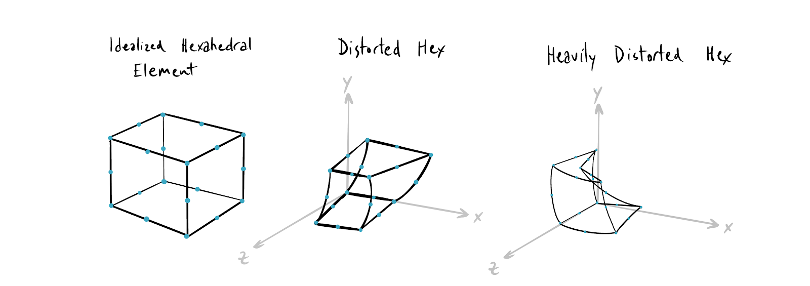
Analyze your mesh to determine locations where the jacobian of elements deviates from that of an undistorted (idealized) element. Use this to guide your mesh refinement.

Stress Gradient Eyeballing

When analyzing results, keep the element lines visible and look for broken color bands between element and large color gradients in individual elements. Large changes are evidence of higher order field variable behavior that would be better represented by more elements.

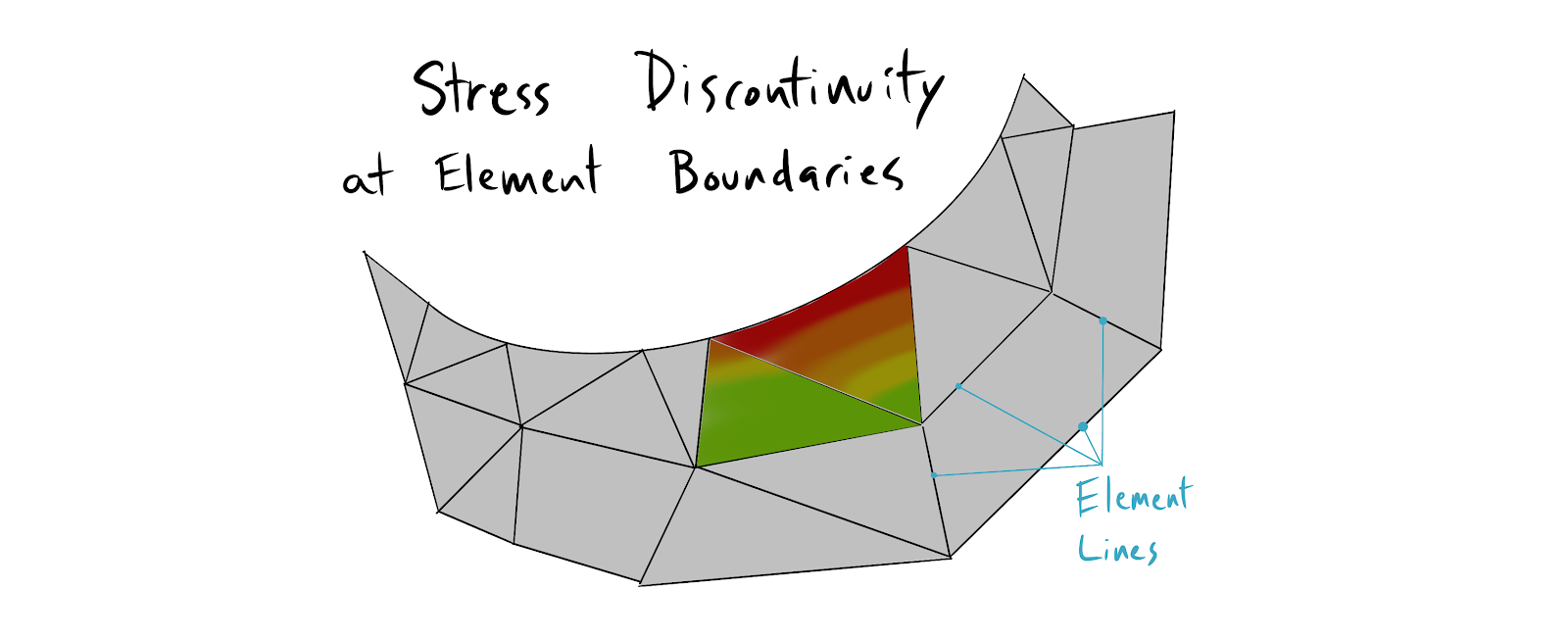
Broken color bands are evidence of displacement, strain, and stress discontinuities which are unlikely to occur in real life continuous materials. Nature has an inherent smoothness which you should look for in your models. Stress flow and heat flow in the real world tend to be C0 and C1 continuous in most cases.

Energy Norm Check

This is effectively the numerical method for checking stress gradients. Element corner stresses meeting at a common node will not have the same value if the mesh is too coarse. The Energy Norm is the work (force x distance) done by this stress discontinuity. If you sum all the node specific energy norms you arrive at a total energy norm due to stress error. Dividing the total energy norm by the total strain energy in the model results in the Global Estimated Error Rate. This rate should be kept as low as possible.

Average vs Unaveraged Element Stress Check

Compare the average ISO stress image to the unaveraged (discontinuous ISO) stress image in your models. Areas of disagreement indicate discretization errors which can often be solved by local mesh refinement.

Convergence Check

Run convergence checks on your models. Many FEA tools have explicit support for convergence checking. You should be modifying your mesh via local (and sometimes global) mesh refinement until you no longer see large percentage changes in model output. This doesn’t guarantee that you have a correct answer because you may have faulty underlying assumptions. However, it does give you some assurance that your finite element representation is consistent with your real world problem as filtered through your particular application of engineering theory.

Boundary Condition Gut Check

Run an animation of displacement to get a better feel for the accuracy of your boundary conditions. This can reveal over and under constraint problems quicker than just looking at a single image of deformed output.

Mesh Smarter

Let CAD guide your meshing, but evaluate the mesh based on your understanding of finite element theory. Remember that most FE codes have no explicit knowledge or internal representation of the geometry being examined. Even the best auto-meshing tools require careful adjustment to get high fidelity results. Only you know where to expect large changes in field variables. Adaptive meshing tools don’t know anything about field variables a priori.

Develop and Use Geometry Specific Meshing Rules of Thumb

Develop your own rules of thumb for meshing and communicate them to your team and colleagues. The following rules serve as a starting place which must be adapted to your specific problems.

For bent flanges and sheet metal components use four elements through the thickness.
Holes should have a minimum of 12 elements around the circumference. If the hole is a potential failure location, use 24 elements or more.
Launch vehicles, pressure vessels and other large cylinders should have a minimum of 72 circumferential elements, or one every 5 degrees.

Don't Trust First Order Elements

You should only be using first order elements (especially tet elements) for initial model setup (ex: proving that your loads, constraints, and material representations are compatible with internal solvers). First order (linear) tet elements grossly overestimate stiffness. Do not rely on first order elements for accurate results.

Hyperelasticity is Challengenging, Proceed with Caution

Hyperelastic materials like rubber are difficult to model for three reasons.

Poisson’s ratio is often near 0.5, leading to volumetric locking and/or greater difficulty in accurately representing stiffness.
Hyperelastic materials are compliant, leading to large displacements.
The difficulty of representing stiffness interacts with the non-linearity of large displacement models to compound errors. It is also difficult to develop intuition for these problems. Physical testing is recommended for large displacement hyperelastic problems.

Use Shells for Thin Features

Default meshing tools in some FEA programs use tetrahedral elements independent of the geometry being analyzed. Tet elements are not good at representing thin wall parts, especially thin walled parts in bending. If you must use tet elements make sure there are several elements through the thickness of the solid.

Flip Boundary Conditions: Swap the Location of Constraints and Loads and Check for Agreement Between Models.

The choice of what features to load and what to constrain is somewhat arbitrary. Inverting which features are loaded vs. constrained and looking for agreement between the two models can help you identify overconstraint problems.

When in Doubt Test Your Way Out

If the accuracy of the analysis is critical and important business decisions are made based on your model’s results, it becomes increasingly important to validate your model empirically. There is no substitute for a real world experiment with the actual system in question.

Takeaways

Perhaps just as important as understanding the theory and mathematical foundation of FEA, it is also important to develop a healthy attitude and respect for FEA as well. It is incredibly powerful precisely because it is complicated and adaptable. FEA is a methodology that will allow you to solve increasingly complex problems while still confronting you with your own ignorance as you learn more. If you want great results it is important to take a long term view of FEA, start small and build simple models you can understand, replicate and trust.

One more thing before you go!

Great hardware product development is all about iterating quickly and learning as much as possible with each iteration. We've built Five Flute to help teams discover and resolve more issues per iteration so you can get to market faster and deliver products that meet your design requirements. If you want to supercharge your product development collaboration check out Five Flute today or sign up for a demo!