What is the Monte Carlo Simulation?

The Monte Carlo Simulation, aka Monte Carlo Method, aka Multiple Probability Simulation, is a powerful computational technique in the mechanical engineer’s toolkit. It’s a computational method that models the statistical probability of various outcomes via a prediction method fueled with random variables.

The Monte Carlo Method applies when there is a high level of uncertainty when forecasting or estimating and the variable with uncertainty can be represented with a random value. There are a number of common applications of the Monte Carlo simulation in engineering (or mechanical engineering), including:

• Statistical tolerance analysis
• Reliability design
• Uncertainty analysis in measurement
• Robotic error, position, and attitude analysis
• Design optimization

Some non-engineering-based applications of the Monte Carlo Method you may be familiar with include:

• asset price projection
• risk of an entity defaulting in the financial world
• risk mitigation in the oil and gas industry
• determining the likelihood of an extreme weather event in meteorology
• determining which stable particles interact in particle physics detectors

In this article, we will focus on building an understanding of Monte Carlo methodology, establishing a framework for analysis that applies to a variety of problems, and applying this framework to a common statistical tolerance analysis problem — our goal is to provide you an easy-to-understand introduction to Monte Carlo Simulations.

Method Overview

The fundamental concept of Monte Carlo methods is to utilize the power of statistical probability and randomness to solve deterministic problems. Consider this example:

Problem Statment: Roll three six-sided dice. How often will the sum of the dice be greater than seven?

The problem itself is deterministic, meaning it has one and only one answer. Dice behave the same way no matter where they are rolled and who rolls them. And yet, there is an element of randomness as well. You cannot predict what any individual die will land on before you roll it. There’s a high probability that your statistics class taught you that. (See what I did there?)

However, it’s easy to see the result of a single dice roll and check against the condition laid out in our problem statement — do they add up to more than seven?

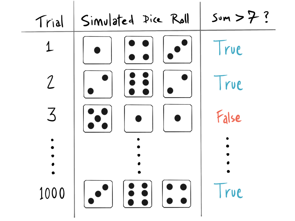
That’s the beauty and power of the Monte Carlo method. There are many problems where computing the answer directly is difficult, but checking the outcome of an “experiment” (in this case a dice roll) is trivial. The method relies on conducting a sufficiently large number of experiments or trials, such that counting the outcome of each trial tells us the answer to the original question in a general sense.

Analysis Framework Fundamentals

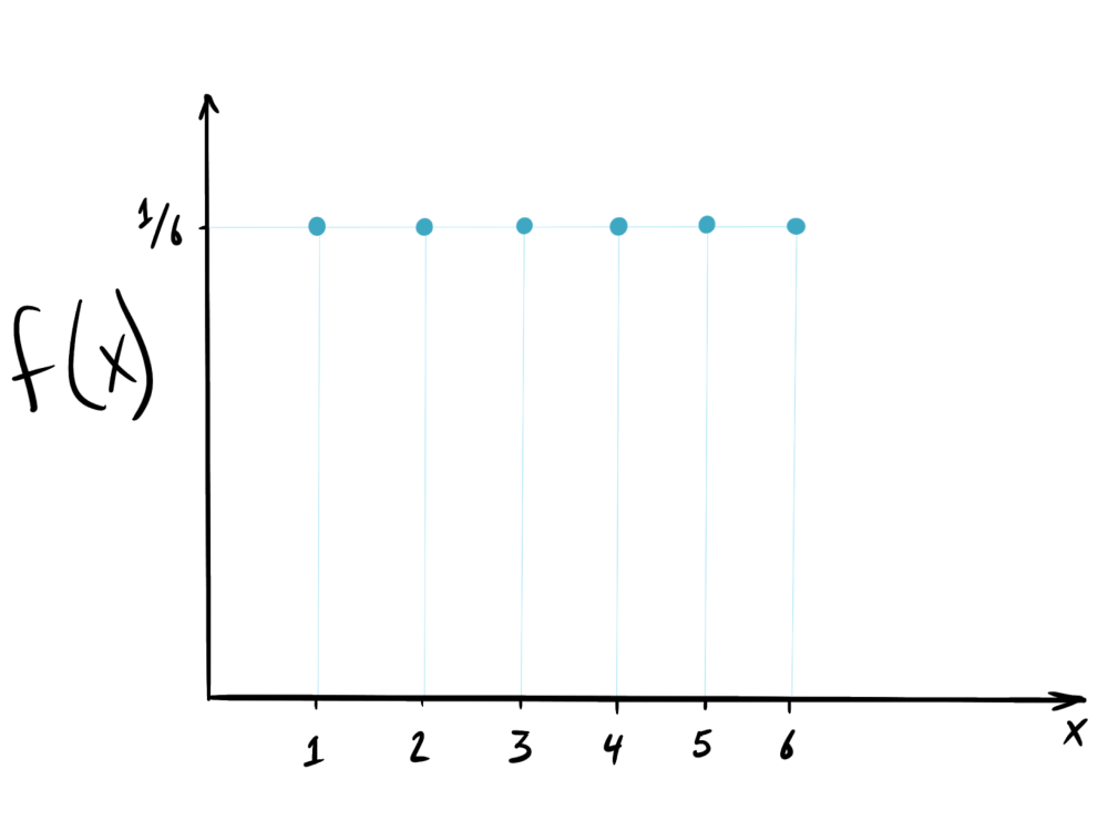
The Probability Density Function (PDF) is a core component of any Monte Carlo simulation. A PDF completely describes the behavior of any random variable that is being simulated. In the dice roll example, the PDF is easy to understand. When you roll a single die, there is an equal (⅙) chance of any number being rolled. This uniform probability density function is plotted below.

In order to construct a useful Monte Carlo simulation, you must use a representative PDF that accurately captures the behavior of each trial in the real world. Unlike dice, the dimensions of mechanical parts and other engineering processes exhibit continuous variability. With continuous random variables, there are an infinite number of values possible even within a finite range. Accordingly, you need a function such as a Gaussian (or normal) distribution to represent continuous random variables accurately.

Example PDF: Gaussian Function

The exact PDF necessary for your analysis depends upon the phenomenon you’re trying to represent and may require some other distribution besides Gaussian (ex: power law, Weibull, Bernouilli, Binomial etc…)

Analysis Framework

Now that we understand the core component of a trial — the probability density function — we can build an analysis framework around it. There are five steps in the framework outlined below. These steps will be explained using pseudocode, as well as references to Google Sheets, MATLAB and python functions you can use in your own applications.

You can construct a useful simulation in spreadsheets or with your programming language of choice as long as you understand the framework and apply it accurately.

1. Construct PDFs. Represent all variables as probability density functions, either discrete or continuous. (ex: multiple normal distributions each with their own independent mean and standard deviation values)
2. Construct functions to sample from these distributions. In google sheets you can use the NORMINV() function combined with RAND() for random sampling. In python you can use the np.random.normal from the numpy package.
3. Construct a trial check function. This function looks at an individual simulation trial and checks the results of that trial against some deterministic outcome. For example, is the sum of the three dice greater than seven (true or false)? This function (or functions) should aggregate and store your individual trial’s results for later use. In excel or g-sheets this usually means constructing a trial results column. In python or MATLAB you should construct a list, tuple, or array (or other data structure) where you store the trial results.
4. Construct a simulation results check function. This function poses your engineering question in such a way that it can be answered by running some computation on the individual trial results. This is where your creativity really comes into play, and it is also where the flexibility and power of the method comes alive. Coming up with creative ways to relate the aggregate trial data to engineering problems is what allows this method to work in so many domains.
5. Construct the main simulation using the following pseudo code as a guide.

    # For each trial (main simulation loop)
       # sample from the relevant probability distribution functions
       # check the samples using your trial check function(s)
       # store the results of each trial check

    # Run the simulation results check function to compute your simulation results

Note that there are numerous other simulation frameworks that you can use for Monte Carlo simulations. Some simple simulations benefit from running the results check function inside the main simulation loop, incrementing results variables after each trial.  The suitability of one framework over the other depends on personal preference and the nature and complexity of the problem being solved.

Monte Carlo Method Tolerance Analysis Example: O-ring compression problem

Suppose we’re designing a hydraulic piston and cylinder actuator that uses buna-n O-rings to seal around the piston (see schematic below).

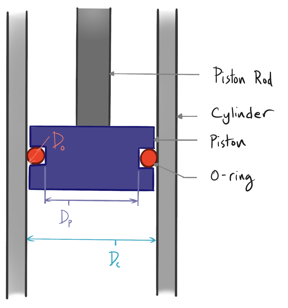
The O-ring is designed to work in a certain interference (compression) range which we will call X.  The cylinder, piston, and O-ring have the following dimensions and manufacturing tolerances.

O-ring diameter = 3mm ±0.09 mm = DO

Cylinder inner diameter = 25mm ±0.1 mm = DC

Piston ring groove diameter =22.5mm ±0.03 mm = DP

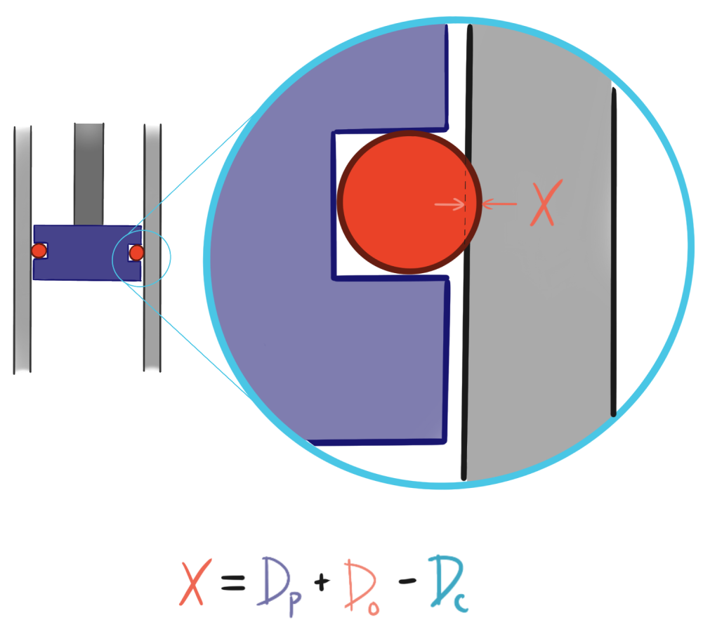
correction: The above equation should read 2X instead of X.

In order for the piston seal to function properly, the O-ring compression must remain between 0.3mm and 0.6mm.  With the above manufacturing tolerances, what percentage of actuators will not be functional?

Solution

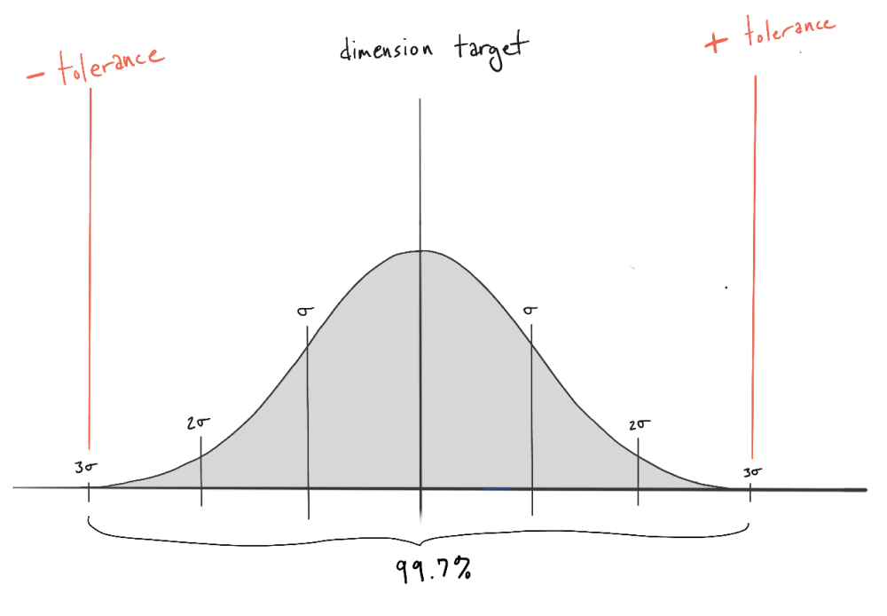
Using our analysis framework we must first choose a PDF to represent each machining process and critical dimension of the assembly. We will use a normal distribution where the mean is the target dimension, and the standard deviation is derived from the specified machining tolerances. A common assumption with these types of tolerancing problems is that the tolerance specified in design is achieved on 99.7% of parts, or a three standard deviation (sigma) coverage.

After choosing our PDFs for each dimension in the tolerance stack, we then sample each distribution to “build an assembly” for each simulation trial. Finally, we check each assembly against our functional O-ring specification and aggregate the results. You can find the Python code for the whole process below.

Python Example Code

import numpy as np
import matplotlib.pyplot as plt

n = 1000000 # number of trials

# Component specifications
sigma = 3       # assume 99.7% of components in tolerance spec
dp = 22.5       # piston diameter
tol_dp = 0.03   # piston diameter tolerance
do = 3          # o ring diameter
tol_do = 0.09   # o ring diameter tolerance
dc = 25         # cylinder diameter
tol_dc = 0.1    # cylinder diameter tolerance


def calculateInterference(dp, do, dc):
    """
    in: diameters
    out: o ring interference 
    """
    
    interference = dp + do - dc
    return interference

def checkInterference(interference, lower, upper):
    """
    in: o ring interference
    out: Bool, T for pass, F for fail
    """
    
    if interference < lower or interference > upper:
        return False
    else:
        return True

# set interference limits
lower = 0.3 # smallest permissable interference 
upper = 0.6 # largest permissable interference
      
interference_list = []  # initialize a list to store interference values per trial 
results = []            # initialize a list to store our trial results

# Main simulation loop
for trial in range(n):
    # Sample PDF for each component
    piston_sample = np.random.normal(dp, tol_dp/sigma)
    oring_sample = np.random.normal(do, tol_do/sigma)
    cylinder_sample = np.random.normal(dc, tol_dc/sigma)
    
    # compute and store interference 
    interference = calculateInterference(piston_sample, oring_sample, cylinder_sample)
    interference_list.append(interference)
    
    # Trial check: log results of interference check
    results.append(checkInterference(interference, lower, upper))

# results check
goodAssemblyCount = sum(results)
failurePercentage =  100*((n - goodAssemblyCount) / n)

print('Percentage of failed piston assemblies: ', failurePercentage, "%")


# Plot results
#setup histogram parameters for plotting
n_bins = 500
heights, bins, _ = plt.hist(interference_list, bins=n_bins) # get positions and heights of bars

bin_width = np.diff(bins)[0]
bin_pos = bins[:-1] + bin_width / 2

# mask for coloring failures differently
maskleft = (bin_pos <= lower)
maskright = (bin_pos >= upper)

# plot data in three steps
plt.figure(figsize=(14, 4))
plt.bar(bin_pos, heights, width=bin_width, color='#281E78', label='Good Assemblies')
plt.bar(bin_pos[maskleft], heights[maskleft], width=bin_width, color='#ea4228', label='left tail failures')
plt.bar(bin_pos[maskright], heights[maskright], width=bin_width, color='#49C6E5', label='right tail failures')

# axis labels and vertical markers of left and right tail failures
plt.xlabel("O ring interference (mm)")
plt.ylabel("# samples")
plt.axvline(lower, linestyle='--',linewidth=1, color='grey')
plt.axvline(upper, linestyle='--',linewidth=1, color='grey')

# remove upper and right spines, set ticks
ax = plt.gca()
ax.spines['right'].set_visible(False)
ax.spines['top'].set_visible(False)
ax.xaxis.set_ticks_position('bottom')
ax.yaxis.set_ticks_position('left')

plt.legend()
plt.show()

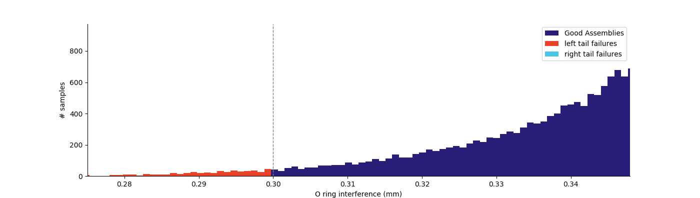
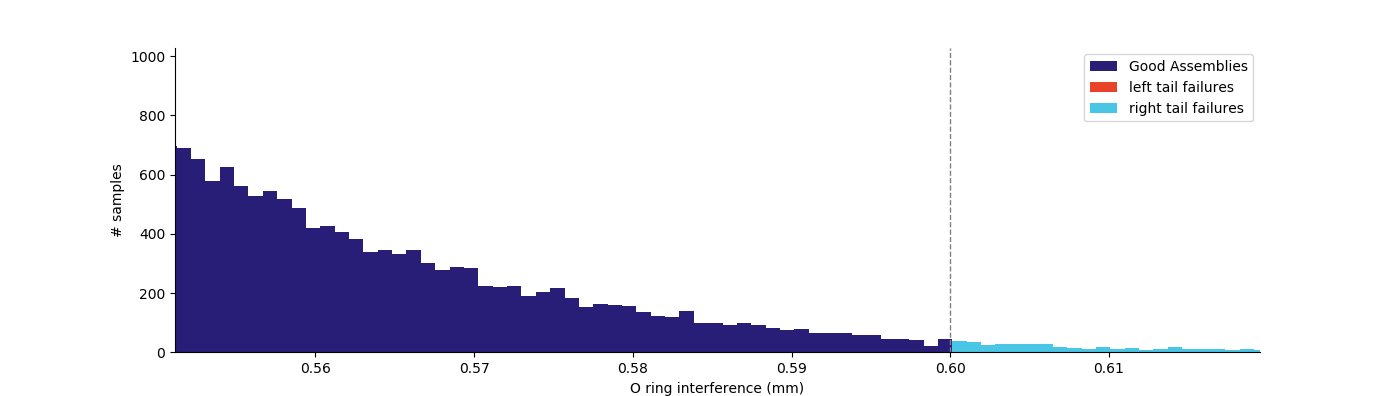
Our one million trial simulation shows a piston assembly failure percentage of 1.4738%.

However, we don’t know the distribution of failures or how we might modify our design to prevent them. To visualize the distribution of O-ring interference, we can plot a histogram of our simulation data with the following code.

The histogram of O-ring interference below shows that all failures are happening on the right tail of the distribution, meaning there’s too much interference.

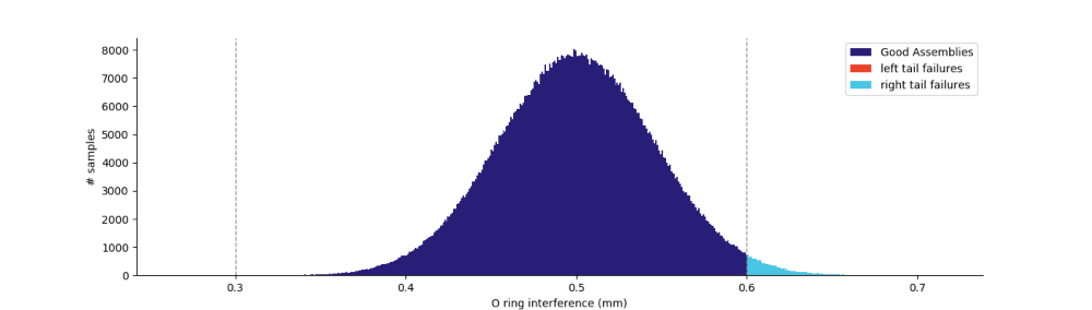
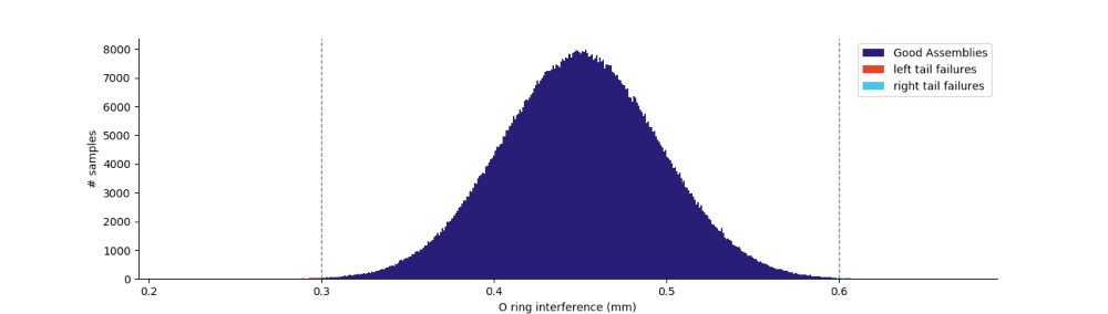
Given that there is room on the left tail of the distribution, a simple fix is to adjust one of the dimensions in the stack up to shift the assembly distribution left.  We can simulate this by reducing the piston ring groove diameter from 22.5mm to 22.45mm while keeping all tolerances the same. Simulating this condition reduces failure to 0.1118% by centering the O-ring interference distribution between the left and right tail cutoffs. You can see the difference below.

Takeaways

The main thing to take away from this post is that the Monte Carlo method is not difficult to implement and can be incredibly flexible and useful for a variety of common mechanical engineering problems. Understanding the basic Monte Carlo framework allows you to quickly create useful simulations in spreadsheets or python code in just a few minutes.

When assessing the accuracy of your simulations, remember these key facts:

• The probability density functions must be representative of the actual system behavior in the real world.
• The samples you draw from the probability density functions must be random samples. Otherwise, your models will not represent the population accurately.
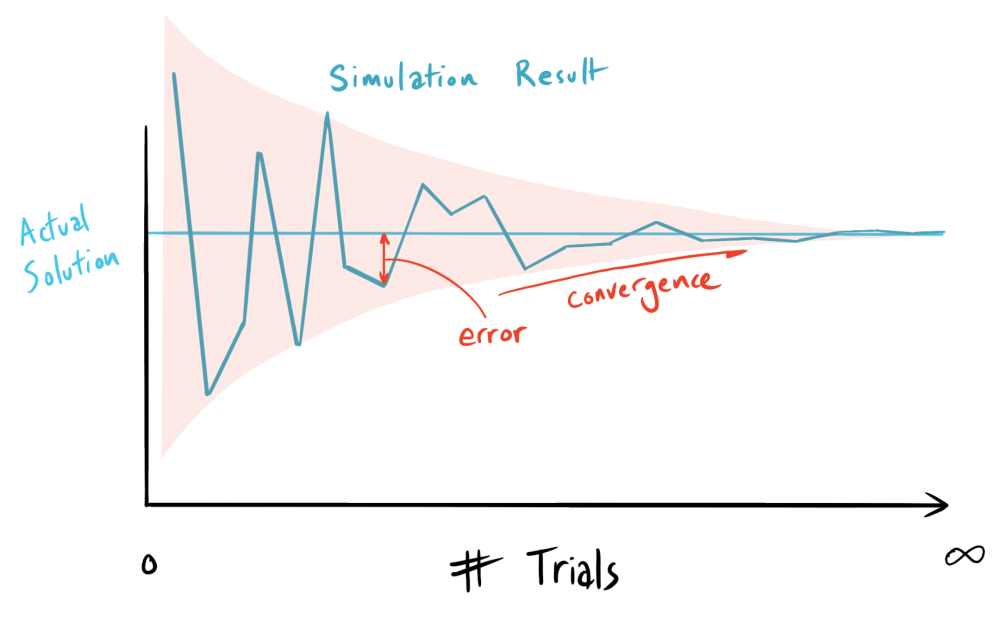
• The law of large numbers dictates that as the sample (trial) count increases, model accuracy increases.
• For models that require highly accurate answers, the trial count should be increased until the accuracy of the simulation no longer changes. Checking convergence does not guarantee that the model is accurate, but it does yield efficient results by allowing you to balance the cost of computation against marginal increases in model accuracy.